Linear Programming Solver with Steps (up to 21 variables)
Linear Programming Solver with Steps
This linear programming solver online (LP solver) helps you solve LP models from a coefficient table and shows steps. Two‑Phase simplex is the default; Exact mode supports fractions.
Need integer/binary decisions? Switch Variable domain to solve ILP/MILP via Branch & Bound. For N=2, use Graphical for a linear programming graph view (boundary lines / corner‑point intuition).
Inputs
Beginner mode adds plain‑English narration plus a verification table (plug the solution into every constraint and bound).
Objective coefficients (c)
Upper bounds (optional)
Enter Uᵢ to enforce xᵢ ≤ Uᵢ. Leave blank for “no upper bound”. Nonnegativity xᵢ ≥ 0 is always assumed. (Upper bounds often fix “unbounded” outputs.)
Advanced (step detail + bulk paste)
Bulk paste (optional)
UB line is optional. Leave a blank entry for “no upper bound”.
Constraints (A x ≤/≥/= b)
Fill coefficients, choose relation, then RHS. Blank coefficients are treated as 0.
Export / share details
Results
—
Step-by-step explanation (standard form + simplex steps)
Steps will appear here after you calculate.
Primal ↔ Dual (dual LP calculator: generate & solve)
Use this to solve the dual of a linear program and check strong duality (when the model is feasible and bounded).
Run a calculation first.
Export full report
Export a complete worked solution (copy/paste friendly).
Choose Word-friendly text to paste into Word. Use HTML for rich formatting.
Chart
If N=2: boundary lines are drawn (graphical method / linear programming graph solver view; corner-point intuition). If N>2: a bar chart of top variables is shown after you solve.
Understanding the results
- Status explains whether the model is feasible and bounded (Optimal / Multiple optimal / Infeasible / Unbounded).
- Z* is the best objective value (maximum or minimum depending on your selection).
- x1…xn are decision variables. Their values are the recommended amounts/levels at the optimum.
- Multiple optimal means there are multiple solutions that achieve the same Z*.
Common mistakes
- Forgetting the calculator assumes xᵢ ≥ 0.
- Swapping ≤ and ≥ signs (changes the feasible region completely for N=2 models).
- Getting Unbounded because real-world caps/limits were not modeled (use upper bounds or additional constraints).
- Choosing integer/binary without tight bounds (Branch & Bound can grow fast). See integrality tolerance and LP relaxation bound.
Limitations
This is a teaching/utility linear programming solver with steps. It does not model nonlinear relationships, uncertainty, or industry-specific feasibility rules. For high-stakes decisions, validate using a production solver and your full constraint set.
Worked examples (copy/paste models)
Tip: Use Advanced → Bulk paste for the fastest input. These examples cover LP, ILP/MILP, ≥/= constraints, upper bounds, unbounded/infeasible cases, exact fractions, and primal–dual learning.
Chapter 1 — Beginner basics (start here): Examples 1–4
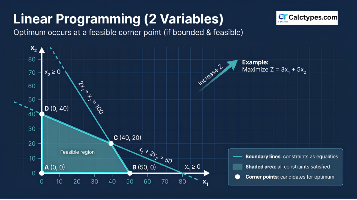
Example 1 (Easy) — Continuous LP (Max) with 2 variables
Goal: Basic LP (continuous). Works well with Graphical (N=2) or Two‑Phase.
- Objective: Maximize
- Variables: N=2
- Constraints: M=2
- Domain: Continuous
Bulk paste
OBJ: 3, 5
C: 2, 1 <= 100
C: 1, 2 <= 80
Expected optimum: x1 = 40, x2 = 20, Z* = 220.
Example 2 (Easy) — Integer LP (ILP) “Workshop” (Branch & Bound)
Decision variables: x1, x2 are units to produce (must be integers).
- Objective: Maximize
- N: 2, M: 2
- Domain: All integer (ILP) → Branch & Bound
Bulk paste
OBJ: 3, 5
C: 2, 1 <= 8
C: 1, 2 <= 8
Expected ILP optimum: x1 = 2, x2 = 3, Z* = 21.
Note: Continuous relaxation would give x1=x2=8/3 (≈2.6667), Z≈21.3333.
Example 3 — 0–1 (Binary) Knapsack (6 variables)
Choose items (xᵢ ∈ {0,1}) to maximize value with one capacity constraint.
- Objective: Maximize
- N: 6, M: 1
- Domain: All binary (0–1)
Bulk paste
OBJ: 24, 13, 23, 15, 16, 12
C: 12, 7, 11, 8, 9, 6 <= 26
Expected optimum: pick items 1,4,6 → x = (1,0,0,1,0,1), Z* = 51.
Example 4 — Minimization with ≥ constraints (Two‑Phase)
≥ constraints require surplus + artificial variables internally → Two‑Phase is appropriate.
- Objective: Minimize
- N: 2, M: 2
- Domain: Continuous
Bulk paste
OBJ: 0.5, 0.2
C: 3, 1 >= 10
C: 1, 2 >= 8
Expected optimum: x1 = 2.4, x2 = 2.8, Z* = 1.76.
Chapter 2 — Features & statuses (Multiple optimal / UB / Unbounded / Infeasible): Examples 5–8
Example 5 — Equality constraint → Multiple optimal solutions
This example is designed to show the status Multiple optimal solutions.
Bulk paste
OBJ: 1, 1
C: 1, 1 = 10
C: 1, 0 <= 7
C: 0, 1 <= 8
Expected: Z* = 10, with infinitely many solutions along x1+x2=10 that respect x1≤7 and x2≤8.
Example 6 — Using Upper bounds Uᵢ (xᵢ ≤ Uᵢ)
Bulk paste (includes UB line)
OBJ: 5, 4
UB: 3, 10
C: 1, 1 <= 100
Here x1 is capped at 3 even though the constraint allows much larger values. Learn more: Upper bounds in linear programming.
Example 7 — Unbounded model (shows “Unbounded” status)
Bulk paste
OBJ: 1, 1
C: 1, -1 >= 0
Expected status: Unbounded. Fix checklist: Unbounded vs infeasible.
Example 8 — Infeasible model (shows “Infeasible” status)
What to enter (use N=2)
OBJ: 1, 0
C: 1, 0 >= 5
C: 1, 0 <= 3
Expected status: Infeasible. Fix checklist: Why LP says infeasible.
Chapter 3 — Advanced methods (MILP / Exact fractions / Duality / Binary switch): Examples 9–12
Example 9 (Advanced / “Hard”) — MILP Facility Opening + Shipping (15 variables, binaries + equalities)
Goal: Show a realistic MILP with: shipping variables (continuous), facility open decisions (binary), equality demand constraints, and linking capacity constraints.
A) Variables (how we map calculator variables)
The calculator uses x1…x15. We interpret them as:
| Calc var | Meaning | Type |
|---|---|---|
| x1..x4 | Ship from Facility 1 to Customers 1..4 (F1→C1..C4) | Continuous ≥0 |
| x5..x8 | Ship from Facility 2 to Customers 1..4 (F2→C1..C4) | Continuous ≥0 |
| x9..x12 | Ship from Facility 3 to Customers 1..4 (F3→C1..C4) | Continuous ≥0 |
| x13 | y1 = 1 if Facility 1 is open | Binary |
| x14 | y2 = 1 if Facility 2 is open | Binary |
| x15 | y3 = 1 if Facility 3 is open | Binary |
B) Data (costs, demands, capacities)
- Demands: C1=20, C2=25, C3=15, C4=30
- Capacities: F1=50, F2=60, F3=40
- Fixed opening costs: F1=200, F2=180, F3=120
- Shipping costs per unit:
F1→(C1..C4) = (2,7,5,9)
F2→(C1..C4) = (6,3,4,4)
F3→(C1..C4) = (5,6,2,7)
C) Mathematical model (what coefficients mean)
- Objective coefficients are costs: each shipping variable has a per-unit cost; each y variable has a fixed cost.
- Demand constraints (=) enforce exact satisfaction: total shipped to each customer equals its demand.
- Capacity linking constraints (≤) enforce: “if yᵢ=0 then facility i ships 0; if yᵢ=1 then it can ship up to its capacity.”
Implemented as: (sum of shipments) − capacity·yᵢ ≤ 0
D) Exactly what to enter in the calculator
- Set Objective = Minimize
- Set Total variables = 15
- Set Total constraints = 7 and click Generate table
- Set Variable domain = Custom
- In Binary indices, enter: 13,14,15 (these are y1,y2,y3)
- Method will auto-switch to Branch & Bound (because binaries exist)
- Use Advanced → Bulk paste with the text below
Bulk paste (complete)
OBJ: 2,7,5,9, 6,3,4,4, 5,6,2,7, 200,180,120
C: 1,0,0,0, 1,0,0,0, 1,0,0,0, 0,0,0 = 20
C: 0,1,0,0, 0,1,0,0, 0,1,0,0, 0,0,0 = 25
C: 0,0,1,0, 0,0,1,0, 0,0,1,0, 0,0,0 = 15
C: 0,0,0,1, 0,0,0,1, 0,0,0,1, 0,0,0 = 30
C: 1,1,1,1, 0,0,0,0, 0,0,0,0, -50,0,0 <= 0
C: 0,0,0,0, 1,1,1,1, 0,0,0,0, 0,-60,0 <= 0
C: 0,0,0,0, 0,0,0,0, 1,1,1,1, 0,0,-40 <= 0
E) Expected optimal solution (so you can verify)
Open facilities: y1=0, y2=1, y3=1 (so x13=0, x14=1, x15=1).
Shipments (nonzero):
| Variable | Meaning | Value |
|---|---|---|
| x6 | F2→C2 | 25 |
| x8 | F2→C4 | 30 |
| x9 | F3→C1 | 20 |
| x11 | F3→C3 | 15 |
| All other x1..x12 | Other shipments | 0 |
Total cost:
Shipping = 25·3 + 30·4 + 20·5 + 15·2 = 75 + 120 + 100 + 30 = 325
Fixed = 180 + 120 = 300
Objective Z* = 625
F) What Branch & Bound is doing (conceptual steps)
- LP relaxation: solves the relaxed model (integer/binary allowed to be fractional) to get a bound.
- Branching: branches on a fractional variable (e.g., y2≤0 and y2≥1).
- Bounding: prunes branches worse than the best integer solution found.
- Termination: proves optimality when all nodes are pruned/solved.
Example 10 — Fraction-heavy LP (Exact rational engine) with exact answers
Goal: Showcase exact fractions (exact rational simplex solver).
Bulk paste
OBJ: 7/3, 5/4
C: 1, 1 <= 5/2
C: 2, 1 <= 4
Expected optimum: x1 = 3/2, x2 = 1, Z* = 19/4 (≈ 4.75).
Example 11 — Dual interpretation (solve primal, then click “Solve the dual”)
Bulk paste (primal)
OBJ: 3, 2
C: 1, 1 <= 4
C: 2, 1 <= 5
Expected primal optimum: x1 = 1, x2 = 3, Z* = 9.
Example 12 (Advanced) — MILP with custom integrality + binary “switch” (linking constraint)
Bulk paste
OBJ: 6, 4, -18
C: 1, 2, 0 <= 14
C: 1, 0, -6 <= 0
Expected optimum: x1 = 6, x2 = 4, x3 = 1 → Z* = 34.
Note: Chapter 3 is long because Example 9 is intentionally a “teaching case”.
Chapter 4 — Higher-level models (Exact + UB / Diet / Assignment / Set cover / Logic / Very hard MILP): Examples 13–18
Example 13 — Fraction-heavy LP (Exact) + Upper bounds (shows exact optimum as fractions)
Purpose: Demonstrate Exact rational engine + upper bounds.
Bulk paste
OBJ: 5/3, 7/4, 9/5
UB: 6, 4,
C: 1, 1, 1 <= 10
C: 1/2, 3/4, 1 <= 8
Expected optimum: x1 = 2, x2 = 4, x3 = 4, Z* = 263/15 (≈ 17.5333)
Example 14 — Diet/Blending (Min) with ≥ constraints (Two Phase) + exact fractional solution
Bulk paste
OBJ: 1/2, 3/10, 2/5
C: 10, 4, 6 >= 50
C: 5, 10, 6 >= 60
Example 15 (Intermediate) — Assignment problem (4×4) as 0–1 ILP (16 binaries)
Bulk paste
OBJ: 9,2,7,8, 6,4,3,7, 5,8,1,8, 7,6,9,4
C: 1,1,1,1, 0,0,0,0, 0,0,0,0, 0,0,0,0 = 1
C: 0,0,0,0, 1,1,1,1, 0,0,0,0, 0,0,0,0 = 1
C: 0,0,0,0, 0,0,0,0, 1,1,1,1, 0,0,0,0 = 1
C: 0,0,0,0, 0,0,0,0, 0,0,0,0, 1,1,1,1 = 1
C: 1,0,0,0, 1,0,0,0, 1,0,0,0, 1,0,0,0 = 1
C: 0,1,0,0, 0,1,0,0, 0,1,0,0, 0,1,0,0 = 1
C: 0,0,1,0, 0,0,1,0, 0,0,1,0, 0,0,1,0 = 1
C: 0,0,0,1, 0,0,0,1, 0,0,0,1, 0,0,0,1 = 1
Example 16 (Advanced) — Set covering (10 binaries, 8 coverage constraints)
Bulk paste
OBJ: 3,4,2,4,1,5,3,3,3,2
C: 1,0,0,0,0,1,0,1,0,0 >= 1
C: 1,1,0,0,0,0,1,0,0,0 >= 1
C: 0,1,0,0,0,1,0,0,1,0 >= 1
C: 0,1,1,0,0,0,0,1,0,0 >= 1
C: 0,0,1,1,0,0,1,0,1,0 >= 1
C: 0,0,0,1,0,1,0,0,0,1 >= 1
C: 0,0,0,1,1,0,0,1,1,0 >= 1
C: 0,0,0,0,1,0,1,0,0,1 >= 1
Example 17 (Advanced) — Project selection with prerequisites + mutual exclusion (binary logic)
Bulk paste
OBJ: 10,8,15,6,12,14,7,9
C: 4,3,7,2,5,6,3,4 <= 15
C: 0,-1,1,0,0,0,0,0 <= 0
C: -1,0,0,0,0,1,0,0 <= 0
C: 0,0,0,1,1,0,0,0 <= 1
Example 18 (Very Hard) — Facility opening + shipping (20 variables, 8 constraints) with full solved optimum
Bulk paste (complete MILP)
OBJ: 2,9,9,9, 4,1,6,6, 6,6,1,4, 9,4,4,1, 250,80,120,200
C: 1,0,0,0, 1,0,0,0, 1,0,0,0, 1,0,0,0, 0,0,0,0 = 30
C: 0,1,0,0, 0,1,0,0, 0,1,0,0, 0,1,0,0, 0,0,0,0 = 20
C: 0,0,1,0, 0,0,1,0, 0,0,1,0, 0,0,1,0, 0,0,0,0 = 25
C: 0,0,0,1, 0,0,0,1, 0,0,0,1, 0,0,0,1, 0,0,0,0 = 15
C: 1,1,1,1, 0,0,0,0, 0,0,0,0, 0,0,0,0, -50,0,0,0 <= 0
C: 0,0,0,0, 1,1,1,1, 0,0,0,0, 0,0,0,0, 0,-30,0,0 <= 0
C: 0,0,0,0, 0,0,0,0, 1,1,1,1, 0,0,0,0, 0,0,-40,0 <= 0
C: 0,0,0,0, 0,0,0,0, 0,0,0,0, 1,1,1,1, 0,0,0,-40 <= 0
Suggestion for learners: start with Chapter 1, then Chapter 2, then Chapter 3–4 for MILP and duality.
Questions people ask
Short answers for students using this LP solver and linear program solver with steps.
Is this a linear programming solver online (LP solver)?
Yes. This is a linear programming solver online (LP solver) that lets you enter coefficients, solve, copy/share results, and export a worked report.
Does this linear programming solver show steps?
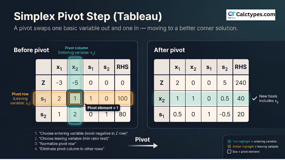
Yes. The Steps panel includes the model, standard-form conversion (slack/surplus/artificial variables), Two‑Phase feasibility logic (W), iteration log, and a verification table in Beginner mode. Learn more: Two‑Phase simplex worked example.
When should I use Two‑Phase simplex vs Big‑M (big m calculator mode)?
Use Two‑Phase simplex when ≥ or = constraints require artificial variables (most reliable). Use Big‑M (decimal) for quick approximate runs (more tolerance‑sensitive). Learn more: Big‑M method step‑by‑step.
Is there a dual simplex calculator mode?
Yes—choose Dual simplex (decimal) when applicable (no artificial variables required). Learn more: dual simplex method example.
How do I get exact fractions (simplex calculator fractions / exact rational simplex solver)?
Choose Exact rational and enter fractions like 5/3. The solver keeps exact arithmetic (helps avoid rounding) and also shows decimals. Try Example 10 in Worked examples.
Does it solve ILP/MILP (ILP solver) with Branch & Bound?
Yes. Set Variable domain to Integer/Binary/Custom to use Branch & Bound. Guides: Branch and Bound in Integer Programming, how to model ILP, ILP beginner’s guide, ILP vs MILP.
Can I use the graphical method (linear programming 2 variables solver)?
Yes. For N=2, Graphical mode draws constraint boundary lines (graph view) to support the corner‑point method intuition. Learn more: Graphical method corner point example.
What does “Unbounded” mean in linear programming?
Unbounded means the objective can improve indefinitely because a real-world cap is missing. Add the missing constraints or use upper bounds. See: unbounded vs infeasible fix checklist.
What does “Infeasible” mean (why does my LP say infeasible)?
Infeasible means no solution satisfies all constraints simultaneously (often a wrong inequality sign, wrong RHS, or contradictory requirements). Beginner mode’s verification table helps you locate the conflict quickly.
Is there a dual LP calculator here (solve the dual of a linear program)?
Yes. Solve the primal first, then open Primal ↔ Dual and click Solve the dual. Learn more: primal and dual linear programming examples.
Do you have a multi objective optimization calculator?
This page solves one objective at a time. For multi‑objective problems, a common LP approach is to combine goals (e.g., weighted sum) into a single objective and solve that LP here.
Advanced topics: optimality gap, Gomory cutting plane, and Model JSON.
Sources
How this calculator works (methodology)
1) What you enter (the mathematical model)
You provide: (a) an objective function (maximize or minimize), (b) constraints of the form A x ≤ b, A x ≥ b, or A x = b, and (c) optional upper bounds xᵢ ≤ Uᵢ. The calculator always assumes xᵢ ≥ 0.
Standard LP form (conceptual):

Max/Min:   Z = cᵀx
Subject to A x (≤, ≥, =) b
           x ≥ 0
Optional:  xᵢ ≤ Uᵢ
2) Standard-form conversion (slack / surplus / artificial variables)
Simplex methods require a starting “basic feasible solution”. To build that, each constraint is converted:
- ≤ constraint: add a slack variable (turns ≤ into =).
- ≥ constraint: subtract a surplus variable and add an artificial variable (to start feasibility).
- = constraint: add an artificial variable (to start feasibility).
Examples:

1) aᵀx ≤ b   ⇒   aᵀx + s = b,   s ≥ 0   (slack)

2) aᵀx ≥ b   ⇒   aᵀx - s + a = b,  s ≥ 0, a ≥ 0  (surplus + artificial)

3) aᵀx = b   ⇒   aᵀx + a = b,   a ≥ 0   (artificial)
3) Two‑Phase simplex (default)
When artificial variables are required, the calculator uses Two‑Phase simplex:
- Phase 1: minimize the sum of artificial variables W. If W* ≠ 0, the model is infeasible.
- Phase 2: optimize your original objective from the feasible basis found in Phase 1.
4) Other modes
- Big‑M (decimal): penalizes artificials heavily; includes a numeric check that artificials are near zero.
- Dual simplex (decimal): works when the tableau is dual-feasible and there are no artificial variables.
- Branch & Bound (integer/binary): solves LP relaxations, then branches on fractional variables to prove an integer optimum.
- Graphical (N=2): enumerates corner points; a verification solve is used to detect unbounded/infeasible cases.
5) Exact vs Decimal engine
- Exact (rational): keeps fractions exactly (best for teaching and accuracy).
- Decimal: faster but uses tolerances (good for quick checks).
6) Why the “Beginner mode” steps are trustworthy
In Beginner mode, the calculator prints a verification table that plugs the solution into every constraint (and bounds / integrality rules).
Visual guides (click to open full size)
These diagrams help you understand the feasible region, simplex pivots, and Branch & Bound.
Related and other calculators
Explore related tools and browse by category. For more optimization tools, visit Operations Research calculators.
VAM / NW corner / least cost + MODI/Stepping Stone optimization with steps.
BMI, calorie, BMR and more—quick tools for everyday decisions.
Algebra, statistics, matrices and more—step-by-step learning tools.
Loans, interest, ROI and planning—fast estimates with clear outputs.