Transportation Problem Calculator with Steps (up to 21×21)
Transportation Problem Calculator
Solve with NW corner, least cost, row/column minima, VAM, Russell, and optional optimization (MODI or Stepping Stone). For large matrices, Results and Step tables are rendered only when you expand/click.
Inputs
Beginner mode adds formulas, VAM penalty tables, MODI/Stepping Stone loop breakdown, and final verification checks.
Bulk paste / import (recommended for large matrices)
Costs: rows separated by new lines; values separated by commas/spaces/tabs. Supply and demand: comma/space separated.
Results
Enter your costs + supply + demand, then click Solve. (Or click Load example.)
Export full report
Export a complete worked solution (copy/paste friendly).
Choose Word-friendly text to paste into Word (no technical skills required). Use HTML for rich formatting.
Embed this calculator
Add this free standards-based calculator to your site — no signup required.
Clicking the button copies an iframe + attribution link (required).
Calculation steps (detailed; tables lazy-load for large matrices)
Steps will appear after you solve. For large matrices, tables are generated only when expanded/clicked.
Understanding the results
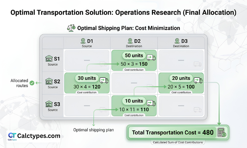
How to Read the Solution (Allocation Table)
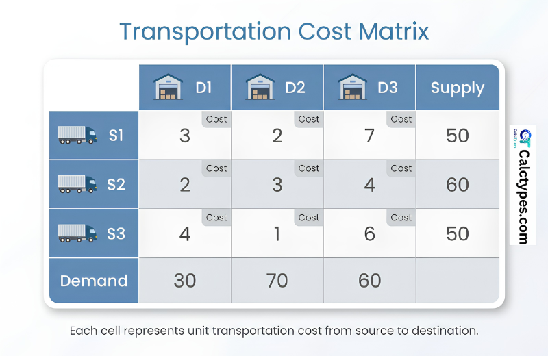
Understanding the Transportation Matrix
- Allocation matrix shows how much to ship from each source to each destination (— means 0 shipment).
- Minimum total cost is computed as ΣΣ(cᵢⱼ × xᵢⱼ) using the balanced matrix used by the solver.
- If the problem is unbalanced, a dummy source/destination is added to balance totals. Dummy shipments are a modeling device and may not represent real routes.
Common mistakes
- Mixing cost units (per-mile vs per-trip vs per-unit) inside the same matrix.
- Treating dummy allocations as real shipments rather than a balancing artifact.
- Turning off optimization and assuming the initial method is always optimal.
Limitations
This solver addresses the classic transportation model. It does not include route capacity constraints, fixed costs, time windows, integer/lot-size restrictions, multi-commodity constraints, or real-world feasibility checks beyond supply/demand balancing. Always validate against your actual constraints.
Questions people ask
Balanced vs unbalanced, initial methods, MODI vs Stepping Stone, degeneracy, and interpreting results.
What does this Transportation Problem Solver calculate?
What is the difference between a balanced and unbalanced transportation problem?
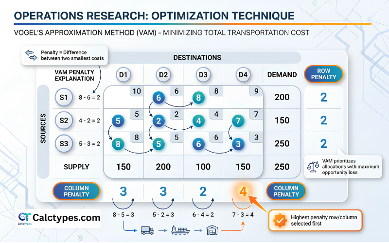
What is Vogel’s Approximation Method (VAM) and why is it recommended?
What is the MODI method in the transportation problem?
What is the Stepping Stone method and how is it different from MODI?
How do I know if my transportation solution is optimal?
What is degeneracy in transportation problems (and what is epsilon ε)?
How is total transportation cost calculated?
How do I paste a large cost matrix from Excel or Google Sheets?
Sources
- Hamdy A. Taha, Operations Research: An Introduction (Pearson). PDF
- Hillier & Lieberman, Introduction to Operations Research (McGraw-Hill). PDF
- Firas Hamid Thanoon, Proposed Method for Solving Transportation Problems. ResearchGate
- Peter Malacký & Radovan Madleňák, Transportation problems and their solutions: literature review. ScienceDirect
- GeeksforGeeks overview (educational). Transportation problem intro
How this calculator works (methodology)
Vogel’s Approximation Method (VAM)
VAM computes penalties (difference between the two smallest costs) for each row and column, then allocates where the penalty is largest.
Method summary
The solver can generate an initial feasible shipping plan using several classic methods (NW corner, least cost, row/column minima, VAM, Russell), and then (optionally) improve/prove optimality using MODI (u–v) or the Stepping Stone method.
Minimize:  Z = ΣΣ (c_ij * x_ij)

Subject to:
  For each source i:      Σ x_ij = s_i
  For each destination j: Σ x_ij = d_j
  x_ij ≥ 0

MODI reduced cost:
  d_ij = c_ij − (u_i + v_j)

Stepping Stone opportunity cost:
  Δ_ij = sum(+c) − sum(−c) along the closed loop through cell (i,j)
Note: In practice, MODI and Stepping Stone identify the same improving moves; they’re two standard ways to test/improve optimality.
Related and other calculators
These calculators are being prepared. They’ll become clickable once published.
Assignment Problem Solver
Optimize one-to-one assignments (often taught alongside transportation problems).
Linear Programming Solver
Solve LP models and understand constraints, objective value, and feasibility.
Minimum Cost Flow Calculator
Network flow optimization for more general routing models.
Simplex Method Calculator
Step-by-step simplex tableaux and optimality interpretation.